"Correlated regressors in multiple regression"
Posted on mars 31, 2014 in misc
It is often asserted that when one two (or more) independent variables are correlated, this creates a problem in multiple linear regression. What problem? And when is it really serious?
In multiple regression, the coefficient estimated for each regressor represents the influence of this regressor when the others predictors are kept constant. Thus it is the “unique” contribution of this variable.
More precisely because the equation is linear:
\(y_{pred} = \beta_0 + \beta_1 x_1 + \beta_2 x_2 + \cdots\)
\(\beta_i\) represents the change in \(y_pred\) when \(x_i\) increases by one unit while the other \(x_j\) remain constant.
When \(x_i\) is orthogonal to all the other predictors, the value of \(\beta_i\) is insensitive to the presence or absence of these predictors in the linear models (assuming that the Ordinary Least Square method is used to estimate the \(\beta\)s). It can still be of interest to include the other predictors in the model if one wants to predict \(y\) or explain out part of the residuals.
If \(x_i\) is not orthogonal to the \(x_j\), \(j \neq i\), then it means that \(x_i\) naturally covaries with them. Then, the meaning of a variation in \(x_i\) when the other are kept constant must be inspected carefully. Take height and weights of humans. An effect of height independant in weight means, for example, that you are going to compare thin tall people with large small ones. This can be interesting, or not. What is crucial is that you are must be able to interpret the coefficients. Sometimes, “all other things being equal” is a pie in the sky.
Now, from a mathematical perspective, unless the predictors are perfectly, or nealry, correlated (the matrix is ill-conditionned), the \(\beta_i\) can be computed without problem.
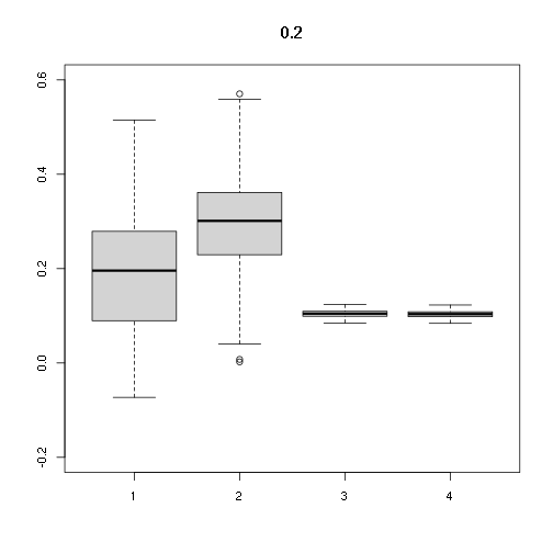
The issues are: - the standard error of these estimates is inflated when correlations becomes high (see the simulations below) - they may be quasi meaningless, especially for predictors that are measured with error.
Let me show an example of the
set.seed(0)
x1 = c(1, 0.9, 0, 0)
x2 = c(0.9, 1, 0, 0)
y = - 3 * x1 + 5 * x2 + rnorm(2, sd=.5)
summary(lm(y ~ x1))
summary(lm(y ~ x2))
summary(lm(y~ x1 + x2))
```gucv
## Error: attempt to use zero-length variable name
require(mvtnorm)
## Loading required package: mvtnorm
require(car)
## Loading required package: car
## Loading required package: carData
n <- 100
a1 <- 0.2
a2 <- 0.3
nsim <- 100
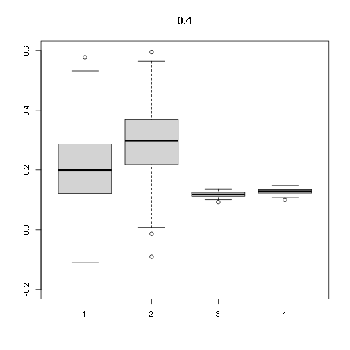
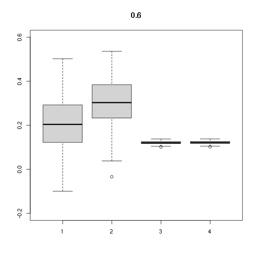
for (cor in c(0, .2, .4, .6, .8))
{
d <- rmvnorm(n, sigma=matrix(c(1, cor, cor, 1), nrow=2))
x1 <- d[,1]
x2 <- d[,2]
print(cor.test(x1, x2))
print("VIF:")
print(vif(lm(rnorm(n)~x1 + x2)))
stats <- matrix(NA, nrow=nsim, ncol=4)
for (i in 1:nsim)
{
y <- a1 * x1 + a2 * x2 + rnorm(n)
lmmod <-lm(y ~ x1 + x2)
slm <- summary(lmmod)
stats[i,] <- as.numeric(slm$coefficients[2:3, 1:2])
}
boxplot(stats, main=cor, ylim=c(-0.2,0.6))
print(apply(stats, 2, summary))
}
##
##  Pearson's product-moment correlation
##
## data:  x1 and x2
## t = -1.6632, df = 98, p-value = 0.09947
## alternative hypothesis: true correlation is not equal to 0
## 95 percent confidence interval:
##  -0.35069101  0.03176625
## sample estimates:
##        cor
## -0.1656857
##
## [1] "VIF:"
##       x1       x2
## 1.028227 1.028227

##               [,1]       [,2]       [,3]       [,4]
## Min.    -0.1111194 0.03887794 0.07899964 0.08409181
## 1st Qu.  0.1169353 0.22843929 0.09521268 0.10134991
## Median   0.2028010 0.29907163 0.09979950 0.10623239
## Mean     0.1923226 0.30571099 0.09964958 0.10607280
## 3rd Qu.  0.2702893 0.38170996 0.10548079 0.11227988
## Max.     0.4542932 0.67791827 0.11671822 0.12424166
##
##  Pearson's product-moment correlation
##
## data:  x1 and x2
## t = 1.5681, df = 98, p-value = 0.1201
## alternative hypothesis: true correlation is not equal to 0
## 95 percent confidence interval:
##  -0.04123689  0.34234645
## sample estimates:
##       cor
## 0.1564484
##
## [1] "VIF:"
##      x1      x2
## 1.02509 1.02509
##                [,1]        [,2]       [,3]       [,4]
## Min.    -0.07293729 0.002299219 0.08478148 0.08395604
## 1st Qu.  0.08970552 0.229864261 0.09911087 0.09814591
## Median   0.19574284 0.301148923 0.10457883 0.10356064
## Mean     0.19334239 0.293744582 0.10433222 0.10331643
## 3rd Qu.  0.27820196 0.360139766 0.10947143 0.10840561
## Max.     0.51454071 0.570414694 0.12410862 0.12290028
##
##  Pearson's product-moment correlation
##
## data:  x1 and x2
## t = 5.564, df = 98, p-value = 2.292e-07
## alternative hypothesis: true correlation is not equal to 0
## 95 percent confidence interval:
##  0.3248046 0.6261254
## sample estimates:
##       cor
## 0.4899642
##
## [1] "VIF:"
##       x1       x2
## 1.315902 1.315902
##               [,1]        [,2]       [,3]      [,4]
## Min.    -0.1099580 -0.09011405 0.09220138 0.1001087
## 1st Qu.  0.1221547  0.22191285 0.11308468 0.1227829
## Median   0.1996379  0.29844973 0.11838175 0.1285343
## Mean     0.2113016  0.29327137 0.11833874 0.1284876
## 3rd Qu.  0.2855133  0.36767892 0.12498448 0.1357033
## Max.     0.5775359  0.59479305 0.13635930 0.1480536
##
##  Pearson's product-moment correlation
##
## data:  x1 and x2
## t = 7.3114, df = 98, p-value = 7.239e-11
## alternative hypothesis: true correlation is not equal to 0
## 95 percent confidence interval:
##  0.4502139 0.7079075
## sample estimates:
##      cor
## 0.594096
##
## [1] "VIF:"
##       x1       x2
## 1.545476 1.545476
##                [,1]        [,2]      [,3]      [,4]
## Min.    -0.09957639 -0.03379669 0.1020250 0.1023815
## 1st Qu.  0.12242156  0.23435938 0.1173215 0.1177314
## Median   0.20420151  0.30328856 0.1208024 0.1212245
## Mean     0.20539909  0.30879211 0.1210283 0.1214512
## 3rd Qu.  0.29252031  0.38150125 0.1257654 0.1262049
## Max.     0.50225276  0.53636922 0.1380224 0.1385047
##
##  Pearson's product-moment correlation
##
## data:  x1 and x2
## t = 15.449, df = 98, p-value < 2.2e-16
## alternative hypothesis: true correlation is not equal to 0
## 95 percent confidence interval:
##  0.7734655 0.8910306
## sample estimates:
##       cor
## 0.8419694
##
## [1] "VIF:"
##       x1       x2
## 3.435393 3.435393
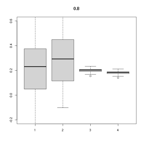
##                [,1]       [,2]      [,3]      [,4]
## Min.    -0.30921893 -0.1007580 0.1546644 0.1403844
## 1st Qu.  0.05129739  0.1156592 0.1920712 0.1743374
## Median   0.23087950  0.2927562 0.2026040 0.1838978
## Mean     0.20684606  0.2865735 0.2009398 0.1823872
## 3rd Qu.  0.37409128  0.4487234 0.2085252 0.1892723
## Max.     0.65650000  0.7602894 0.2330733 0.2115538